When Bigger Models Generalize Better: The Double Descent Phenomenon

Jun 25, 20266 min readmachine-learning, generalization, theory

Originally published on LinkedIn on June 25, 2026. Adapted and expanded here with the underlying math — draft, needs a pass against the original before publishing.

Classical statistical learning theory has a clear warning: past a certain capacity, models stop learning and start memorizing. Add more parameters than you have data, and test error should climb as the model fits noise instead of signal. This is the textbook bias-variance trade-off — a U-shaped curve in model capacity, with a single optimum somewhere short of the point where the model can perfectly fit its training data.

Deep networks routinely violate this warning on purpose. They’re trained with far more parameters than examples, driven to fit the training set essentially exactly, and still generalize — often better than smaller models that stop short of interpolation. Either the bias-variance story is wrong, or it’s incomplete. It’s the latter, and the missing piece has a name, a formal hypothesis, and — in at least one clean special case — an exact closed-form answer.

The classical picture, in one equation

For a model $\hat f$ predicting a target $y = f(x) + \varepsilon$ with noise variance $\sigma^2$ , the expected squared prediction error decomposes as

\mathbb{E}\left[(y - \hat f(x))^2\right] = \underbrace{\left(\mathbb{E}[\hat f(x)] - f(x)\right)^2}_{\text{bias}^2} + \underbrace{\mathrm{Var}(\hat f(x))}_{\text{variance}} + \sigma^2 .

The classical story is that bias falls and variance rises as capacity grows, and the U-shape is just that trade-off. It’s a good story for models with far fewer parameters than data. It says nothing about what happens once the model has enough parameters to drive training error to zero — because in the classical regime, that point is never reached.

Effective model complexity, and where the second curve comes from

Nakkiran, Kaplun, Bansal, Yang, Barak, and Sutskever formalize “how big is the model” not by parameter count but by what it can actually fit. Their Effective Model Complexity (EMC) of a training procedure $\mathcal{T}$ , with respect to a distribution $\mathcal{D}$ and tolerance $\epsilon$ , is

\mathrm{EMC}_{\mathcal{D},\epsilon}(\mathcal{T}) := \max \lbrace\ n \mid \mathbb{E}_{S \sim \mathcal{D}^n}[\mathrm{Error}_S(\mathcal{T}(S))] \le \epsilon \ \rbrace,

the largest sample size on which $\mathcal{T}$ can still drive training error below $\epsilon$ on average. Their Generalized Double Descent hypothesis then splits behavior into three regimes relative to the number of training samples $n$ :

Under-parameterized ( $\mathrm{EMC} \ll n$ ): increasing effective complexity decreases test error — the classical regime.
Critically parameterized ( $\mathrm{EMC} \approx n$ ): increasing complexity can decrease or increase test error — this is the peak, the interpolation threshold.
Over-parameterized ( $\mathrm{EMC} \gg n$ ): increasing effective complexity decreases test error again — the second descent.

This is a hypothesis about any training procedure — deep nets included — but it doesn’t yet say why the critical point is bad or why the second descent recovers. For that, a special case with an exact answer helps.

A special case you can actually solve: linear regression

Hastie, Montanari, Rosset, and Tibshirani analyze the cleanest possible instance: linear regression, $p$ features, $n$ samples, isotropic Gaussian features, fit by ordinary least squares when $p < n$ and by the minimum-norm interpolating solution when $p > n$ (the natural choice among the infinitely many solutions that fit the data exactly). Let $\gamma = p/n$ be the parameters-per-sample ratio — the direct analogue of “how overparameterized is the model.”

For the null case (true signal $\beta_0 = 0$ , so the model is fitting pure noise with variance $\sigma^2$ ), their Theorem 1 gives the asymptotic risk in closed form:

For $\gamma < 1$ (underparameterized):

R(\gamma) = \dfrac{\sigma^2 \gamma}{1 - \gamma}

For $\gamma > 1$ (overparameterized, minimum-norm interpolation):

R(\gamma) = \dfrac{\sigma^2}{\gamma - 1}

Plotted, this is double descent, exactly:

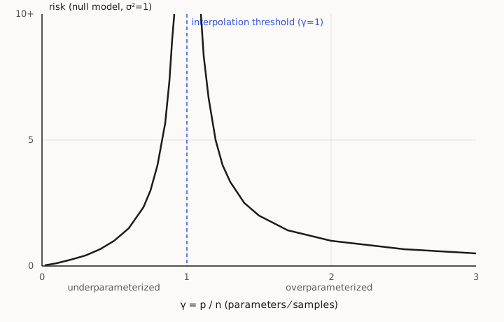
Plot of the null risk R(gamma) = sigma^2 gamma/(1-gamma) for gamma<1 and sigma^2/(gamma-1) for gamma>1, showing risk diverging at the interpolation threshold gamma=1 and decaying back toward zero as gamma grows past 1

Risk of the minimum-norm interpolator as a function of $\gamma = p/n$ , for the null-signal case with $\sigma^2 = 1$ . Diverges at the interpolation threshold and decays back toward zero in the overparameterized regime — this is Hastie et al.’s Theorem 1, plotted directly.

Both branches diverge as $\gamma \to 1$ , exactly at the interpolation threshold, and both decay away from it — the left branch toward $0$ as $\gamma \to 0$ , the right branch toward $0$ as $\gamma \to \infty$ . When there’s real signal ( $\lVert\beta_0\rVert^2 = r^2 > 0$ ), the same theorem gives the overparameterized branch as $R(\gamma) = r^2(1 - 1/\gamma) + \sigma^2/(\gamma - 1)$ — a bias term that saturates at $r^2$ plus the same variance spike, so the qualitative shape survives: sharp peak at $\gamma=1$ , decay on both sides.

Why the peak: a near-singular design matrix

The mechanism behind the spike is concrete, not mysterious. For $\gamma$ just below $1$ , OLS variance scales with $(X^\top X)^{-1}$ , and as $p \to n$ the $p \times p$ Gram matrix $X^\top X$ approaches singularity — its smallest eigenvalues go to zero, and the inverse blows up. For $\gamma$ just above $1$ , the minimum-norm solution instead depends on $(XX^\top)^{-1}$ , and the same thing happens from the other side as $n \to p$ . Right at $\gamma = 1$ , the model has exactly enough capacity to fit the data in only one way, and that one way is maximally sensitive to the specific noise draw it happened to see. This is literally the worst point to be at, and the formula says so quantitatively.

Why the second descent: implicit bias and benign overfitting

Past the threshold, there are infinitely many parameter settings that fit the training data exactly — the system is underdetermined. Minimum-norm least squares always picks the one with smallest $\ell_2$ norm, and it’s this particular selection — not overparameterization by itself — that drives the risk back down. Bartlett, Long, Lugosi, and Tsigler characterize exactly when this works in general linear regression: benign overfitting happens when there are many low-variance directions in parameter space — directions the covariance structure of the features barely uses — for the label noise to hide in, with negligible cost to the prediction. The interpolator perfectly fits the noise, but it fits it into directions that don’t matter.

That’s the real content behind “the model is big enough, so it can afford to memorize the noise without it costing anything.”

Takeaway

The practical shift this implies: stop treating raw parameter count as the thing to regularize against, and start treating the training procedure’s implicit bias as the thing that actually determines generalization once you’re past the interpolation threshold. A model with more parameters than data isn’t doomed — what determines whether it generalizes is whether the optimizer, architecture, and training procedure steer it toward one of the many interpolating solutions that happens to be simple, rather than one that isn’t.

References

Belkin, M., Hsu, D., Ma, S., & Mandal, S. (2019). Reconciling modern machine-learning practice and the classical bias–variance trade-off. PNAS.
Nakkiran, P., Kaplun, G., Bansal, Y., Yang, T., Barak, B., & Sutskever, I. (2019). Deep Double Descent: Where Bigger Models and More Data Hurt. arXiv:1912.02292.
Hastie, T., Montanari, A., Rosset, S., & Tibshirani, R. J. (2019). Surprises in High-Dimensional Ridgeless Least Squares Interpolation. arXiv:1903.08560.
Bartlett, P. L., Long, P. M., Lugosi, G., & Tsigler, A. (2020). Benign Overfitting in Linear Regression. arXiv:1906.11300.

TODO (before publishing): check this against the original LinkedIn text for anything lost in extraction/tone, and confirm the arXiv links resolve to the exact versions you intend to cite.